Automatic physical inference with information maximising neural networks
(Some of this text is directly taken from the our original manuscript, please check it out for all the details)
On this page... (hide)
1. Context
Current data analysis techniques in astronomy and cosmology often involve reducing large data sets into a collection of sufficient statistics. There are several methods for condensing raw data to a set of summaries. Amongst others, these methods could be: principal component analysis (PCA); statistics including the mean, covariance, and higher point functions or; calculating the autocorrelation or power spectrum. Unfortunately, summaries calculated using the above methods can still be infeasibly large for data-space comparison. For example, analysis of weak lensing data from the Euclid and the Large Synoptic Survey Telescope (LSST) photometric surveys will have around {$10^4$} summary statistics. Reducing the number of summaries further results in enormous losses in the information available in the raw data.
Compressing large data sets to a manageable number of summaries that are informative about the underlying parameters vastly simplifies both frequentist and Bayesian inference. When only simulations are available, these summaries are typically chosen heuristically, so they may inadvertently miss important information. A typical compression scheme in large scale structure surveys is to compute a power spectrum of galaxy density fluctuations.
2. Our method
2.1 The general scheme
To achieve a non-linear optimal compression we need two ingredients: a generic way to generate a projection operation (i.e. data to compressed summary) and a reward for choosing that specific function. For the first item, we opt for artificial neural network, which is an adequate tool to generate parametrised arbitrary functions. As for the second item we will set our foundation on the use of the Fisher information.
The use of the Fisher information ensures that we are able to extract the maximal information from data about parameters of interest with reasonable generic assumptions. The neural network needs be trained on artificial data sets to uncover ways to extract the information. To achieve this, we simply need simulations of real data at a fiducial parameter (and the derivative of the simulation with respect to the model parameters). With the compressed summaries, we can then perform likelihood-free parameter inference in the same parameter space as the number of model parameters, rather than the dimension of the data or some heuristically chosen summaries.
2.2 Fisher information and classic MOPED scheme
To begin with, we consider the Fisher information {$$ \tag{1}{\bf F}_{\alpha\beta}(\boldsymbol{\theta}) = -\left\langle\frac{\partial^2\ln\mathcal{L}({\bf d}|\boldsymbol{\theta})}{\partial\theta_\alpha\partial\theta_\beta}\right\rangle.$$} The Fisher information descsribes how much information some data, {${\bf d}$}, contains about some model parameters, {$\boldsymbol{\theta}$}, where the data is described by a likelihood {$\mathcal{L}({\bf d}|\boldsymbol{\theta})$}. In particular, the minimum variance of an estimator of a parameter, {$\hat{\boldsymbol{\theta}}$}, is given by the Cramér-Rao bound {$$\left\langle(\theta_\alpha-\langle\theta_\alpha\rangle)(\theta_\beta-\langle\theta_\beta\rangle)\right\rangle\ge\left({\bf F}^{-1}\right)_{\alpha\beta}$$} such that finding the maximum Fisher information provides the minimum variance estimators of {$\boldsymbol{\theta}$}.
Generally the number of parameters {$n_{\boldsymbol{\theta}}$} is much less than the size of the data {$n_{\bf d}$}. Under the assumption of of Gaussian likelihood {$$ \tag{2}-2\ln\mathcal{L}({\bf d}|\boldsymbol{\theta}) = ({\bf d}-\mu(\boldsymbol{\theta}))^T{\bf C}^{-1}({\bf d}-\mu(\boldsymbol{\theta})) + \ln|2\pi{\bf C}|$$} massively optimised parameter estimation and data (MOPED) compression can be performed which is lossless in the sense that the Fisher information is conserved. In equation (2), {$\mu(\boldsymbol{\theta})=\boldsymbol{\mu}$} is the mean of the model given parameters {$\boldsymbol{\theta}$} whilst {${\bf C}$} is the covariance of the data (and is assumed to be independant of the parameters here). Analytically, the Fisher information can be calculated using equation (1) {$$ \tag{3}{\bf F}_{\alpha\beta} = {\rm Tr}\left[\boldsymbol{\mu},_\alpha^T{\bf C}^{-1}\boldsymbol{\mu},_\beta\right].$$}
The MOPED compression works by transforming the data using {$$x_\alpha = {\bf r}_\alpha^T{\bf d}$$} where {$\alpha$} labels the parameter and {${\bf r}_\alpha$} is calculated by maximising the Fisher information ensuring that {${\bf r}_\alpha$} is orthoghonal to {${\bf r}_\beta$} where {$\alpha\ne\beta$}. The form of {${\bf r}_\alpha$} is {$${\bf r}_1 = \frac{{\bf C}^{-1}\boldsymbol{\mu},_1}{\sqrt{\boldsymbol{\mu},_1^T{\bf C}^{-1}\boldsymbol{\mu},_1}}$$} for the first parameter, {$\theta_1$}, where {$,_\alpha\equiv\partial/\partial\theta_\alpha$}. Each following parameter is transformed using {$${\bf r}_\alpha = \frac{{\bf C}^{-1}\boldsymbol{\mu},_\alpha-\sum_{i=1}^{\alpha-1}(\boldsymbol{\mu},_\alpha^T{\bf r}_i){\bf r}_i}{\sqrt{\boldsymbol{\mu},_\alpha^T{\bf C}^{-1}\boldsymbol{\mu},_\alpha-\sum_{i=1}^{\alpha-1}(\boldsymbol{\mu},_\alpha^T{\bf r}_i)^2}}.$$} As mentioned, the transformation from {${\bf d}\to{\bf x}$} through MOPED compression is lossless under a Gaussian likelihood assumption such that equation (3) is recovered.
So, we have a method to optimally compress data to some sufficient statistics under the condition that the likelihood is Gaussian. However, how do we optimally compress data when the likelihood is not Gaussian or is not known?
2.3 The information maximising neural network (IMNN) scheme
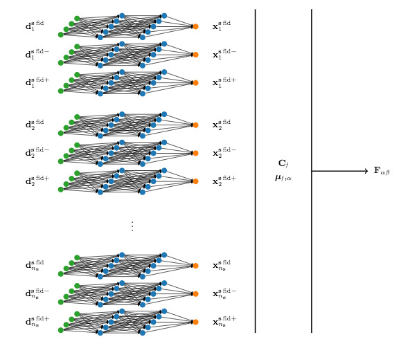
Figure 1: Cartoon of the information maximising neural network architecture. During training, each simulation {${\bf d}^{{\bf s},{\rm fid}}_i$} alongside its fluctuation according to a fiducial parameter (indicated by {$\pm$}) is passed through the same network for which all the weights and biases are shared. The output of the network for each simulation, indicated by {$\bf x$} is used to calculate the covariance, {${\bf C}_f$}, and each of the network outputs from the varied simulations are used to calculate the derivative of the mean output, {$\boldsymbol{\mu}_f,_\alpha$}. Once trained, a summary of some data can be obtained using a simple artificial neural network with the weights and biases from the training network.
We consider an unknown non-linear map from the data to a set of compressed summaries {$f:{\bf d}\to{\bf x}$}. This function should be chosen such that the likelihood is transformed into the form {$$-2\ln\mathcal{L}({\bf x}|\boldsymbol{\theta}) = ({\bf x}-\mu_f(\boldsymbol{\theta}))^T{\bf C}_f^{-1}({\bf x}-\mu_f(\boldsymbol{\theta}))$$} where {$$\mu_f(\boldsymbol{\theta}) = \frac{1}{n_{\bf s}}\sum_{i=1}^{n_{\bf s}}{\bf x}_i^{\bf s}$$} is the mean value of {$n_{\bf s}$} summaries obtained from simulations, {${\bf d}_i^{\bf s} = {\bf d}^{\bf s}(\boldsymbol{\theta}, i)$}, by applying the function {$f:{\bf d}_i^{\bf s}\to{\bf x}_i^{\bf s}$}. Each {$i$} denotes a different random initialisation of a simulation. Similarly {${\bf C}^{-1}_f$} is the inverse of the covariance matrix which is again obtained from simulations of the data {$$({\bf C}_f)_{\alpha\beta} = \frac{1}{n_{\bf s}-1}\sum_{i=1}^{n_{\bf s}}({\bf x}_i^{\bf s}-\boldsymbol{\mu}_f)_\alpha({\bf x}_i^{\bf s}-\boldsymbol{\mu}_f)_\beta$$} where {$\boldsymbol{\mu}_f=\mu_f(\boldsymbol{\theta})$}. Using equation (1) we get an updated version of the Gaussian Fisher information in equation (3) {$$ \tag{4}{\bf F}_{\alpha\beta} = {\rm Tr}\left[\boldsymbol{\mu}_f,_\alpha^T{\bf C}_f^{-1}\boldsymbol{\mu}_f,_\beta \right]$$} where {$\boldsymbol{\mu}_f,_\alpha$} and {${\bf C}_f^{-1}$} are calculated at fixed fiducial parameter values, i.e. they are calculated using simulations created at {${\bf d}_i^{{\bf s}~{\rm fid}}={\bf d}^{\bf s}(\boldsymbol{\theta}^{\rm fid}, i)$}.
Our one remaining problem is how to find the unknown function {$f$}. We can use artificial neural networks to learn {$f$} since they are simply a non-linear map from some inputs to some outputs, which is exactly what we need. We consider the data, {${\bf d}$}, (or simulations of the data, {${\bf d}_i^{\bf s}$}) as the network inputs and the outputs of the network as the summaries, {${\bf x}$} (or {${\bf x}_i^{\bf s}$}). By doing this the output summaries are no longer just functions of the parameters, {$\boldsymbol{\theta}$}, and the random initialisation parameter, {$i$}, but also the weights and biases of the network, {${\bf w}^l$} and {${\bf b}^l$}. This means that the means and covariances of the summaries are also functions of the weights and biases, and therefore so is the Fisher information. We can train the network by defining the square determinant of the Fisher information matrix {$$\Lambda = -\frac{1}{2}|{\bf F}|^2$$} as the reward (loss) function, which needs to be maximised.
3. Some application to astronomical datasets
We present two applications of this technique to astronomical datasets: the Lyman-α forest which probes density fluctuations through absorption a strong quasar emission line, and gravitational wave central frequency characterisation.
3.1 Lyman-α forest
The QSOs (quasi-stellar object) produces a strong Lyman-α emission. Coupled with the expansion of the Universe, this emission is redshifted and can be absorbed by other clouds of hydrogen along the line of sight. This absorption is related, in a highly non-trivial way, to the density {$\rho$} at that point. A typical relation is called the "fluctuating Gunn-Peterson approximation" (FPGA) and takes the form: {$$ \tau \propto \rho^{2 - 0.7 \gamma}, $$} for which {$\tau$} is the logarithm of the absorption and {$\gamma$} depends on the physical properties of the intervening gas. In practice the details are even more non-linear and simulations are required to assess the exact relation between the two above quantities. At the same time, cosmology lurks in the auto-correlations of the density {$\rho$} which makes this problem a perfect case-study for our IMNN method. We show in figure 2 a simulated Lyman-α spectrum, generated using classical recipes coming both from observations and simulations.
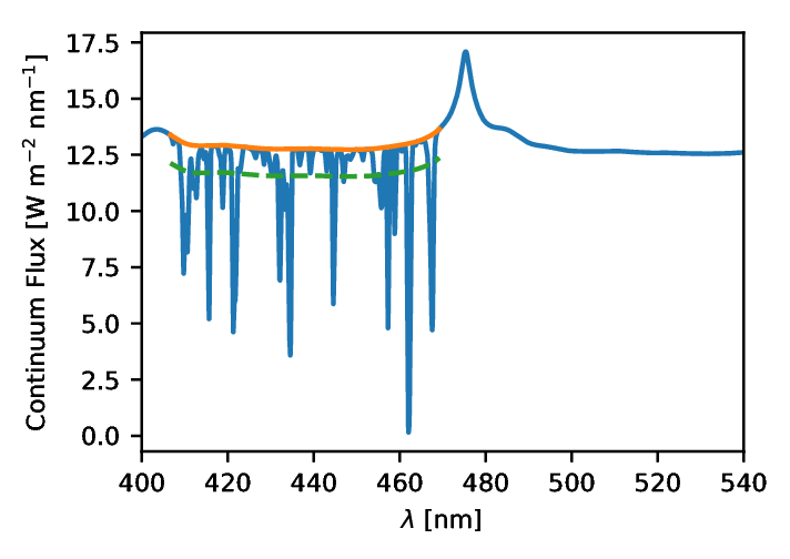
Figure 2: An example of simulated Lyman-α spectrum generated from recipes derived from a set of QSOs observations. On top of the Lyman emission we have added a randomly generated absorption incorporating cosmological information in its correlations.
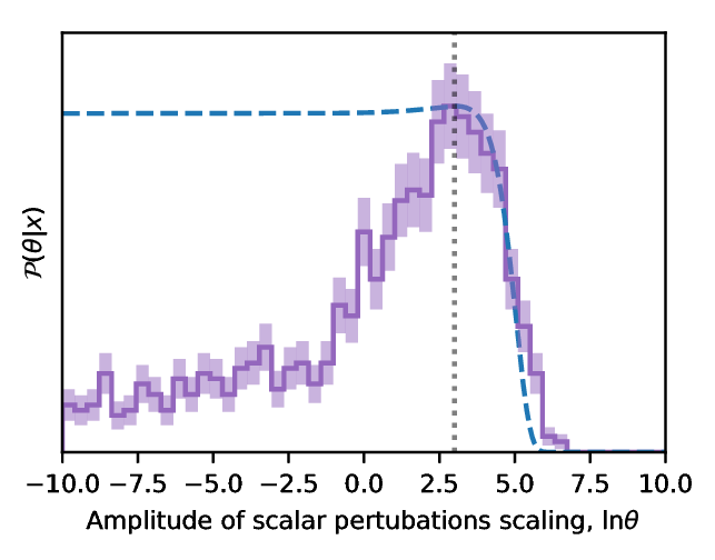
Figure 3: Result of the Approximate Bayesian computation obtained through the information maximisating neural network. We show the probability distribution function of the amplitude of the cosmological powerspectrum as derived from one QSO spectrum. The distribution is very broad but it peaks at the value used in input of the algorithm.
In figure 3 we show the result of parameter inference using the IMNN. We choose to predict the amplitude of scalar perturbations, {$A_{\rm s}$}, which affects the auto-correlation of the density field. To show how the IMNN compression scheme is resistant against poor choice of fiducial parameter we choose the "true" data to have an amplitude of scalar perturbations approximately 20 times larger than in the fiducial training simulations, {$A_{\rm s}^{\rm true} = \theta A_{\rm s}^{\rm fid}$} with {$\theta = \exp(3)$}. The parameter inference of the amplitude of scalar perturbations using only one QSO spectra is shown in figure 3. The posterior distribution peaks at the "true" value of {$\ln\theta=3$} showing that the network has correctly learned the compression scheme for this problem, and not just learned how to pull out information at the fiducial parameter value. This shows us that not only is the IMNN algorithm able to successfully undo extremely-complex non-linear functions from data to parameter, but that it is also capable of being resiliant against weak choices of fiducial parameter.
3.2 Gravitational wave detection
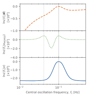
Figure 4: Logarithm of the likelihood for the central oscillation frequency, {$f_{\rm c}$}. The dashed orange line in the upper panel shows the likelihood using all the data, whilst the green dotted line in the middle panel and the blue solid line in the bottom panel show the approximate Gaussian likelihoods when using compression, MOPED and IMNN respectively. All three likelihoods have peaks at the correct {$f_{\rm c}^{\rm true}=0.1$}Hz, but an aliasing peak arises in the MOPED likelihood due to a none-monotonic mapping from {${\bf h}(f_{\rm c})\to x_{\rm MOPED}^{{\bf h}}(f_{\rm c})$}. The compression using the IMNN on the other hand does not have any aliasing peaks since the network has learned the non-linear map from data to frequency.
The IMNN is also able to correctly undo Fourier transform-like functions, which is a problem which cannot be dealt with when using the MOPED compression directly. An illuminating example of this type of problem is seen when predicting the central oscillation frequency of gravitational waveforms. If the frequency space waveform is described as {$$\overline{h}(f) = \frac{AQ}{f}\exp\left[-\frac{Q^2}{2}\left(\frac{f - f_{\rm c}}{f_{\rm c}}\right)^2\right]\exp\left[2\pi i f_{\rm c}t_{\rm c}\right],$$} with noise from the one-sided power spectral density of the LISA detector, {${\bf n}$}, which is assumed to be independent of the signal, then a simple form of the likelihood can be written as {$$ \tag{5}\ln\mathcal{L} = C - \frac{||{\bf d} - {\bf h}(\boldsymbol{\theta})||^2}{2},$$} where {${\bf d} = {\bf h}(\boldsymbol{\theta}^{\rm true}) + {\bf n}$} where {${\bf h}$} is the real space (Fourier-transformed) waveform.
We are interested inferring the value of the central oscillation frenquency {$f_{\rm c}$} where the "true" value is {$f_{\rm c}^{\rm true}=0.1Hz$}. The orange dashed line in the top panel of figure 4 shows the result of (5) using the full data. There is a single peak in the distribution at the true parameter value. However, when using the MOPED compression {${\bf h}\to x^{\bf h}$}, an aliasing peak arises at around {$f_{\rm c}=0.03Hz$}. This forms because the map from the data to the compressed summary is not single valued. On the other hand, when using the IMNN to compress the data, no aliasing peak appears, indicating that the map from data to summary is not degenerate anymore according to the central frequency. This means that when we do parameter inference we do not need to worry about spurious features appearing due to the compression.
4. References
T. Charnock, G. Lavaux, B. D. Wandelt, 2018, Physical Review D 97, 083004, arXiV:1802.03537