BORGModel
On this page... (hide)
1. Generic forward model problem
In BORG, we have to relate the initial density field {$ \delta^{ic} $} to the final matter density fiuctuations {$ \delta^m $}. These two can be formally related by a complex, differentiable, function: {$$ \delta^m_p = F_p\left(\{ \delta^{ic}_q \}\right)\,, $$} with {$ p $} the final grid element label, and {$q$} the initial grid element label. This is a very complex inference problem to solve. Taken at face value, this involves at least a few million dimensions as the grid dimensions are order 1283 (thus ~1 million elements), but generally we are more interested in at least 2563 elements. If we use a classic Markov Chain algorithm, based purely on Metropolis Hasting, then we would do an random walk in 2563 dimensions, among which only one direction gives an improvement of the solution.
In the case of linear data model such as ARES, an analytic solution exists (see ARES). However for this generic problem nothing like that is possible. The only resource is that we can compute the derivative of the function of interest to indicate which direction is most favorable. In BORG, we are in such cases for which we have to deal with a log-posterior {$\psi = \log \Psi$} involving the aforementioned non-linear model: {$$ \psi(\{\delta^{ic}_q\}) = L \circ B \circ F (\{\delta^{ic}_q\})\,, $$} with {$L$} the likelihood, giving metric between the prediction of the model and the data, {$B$} a bias function that remaps the matter density field to observed fields, {$F$} the above non-linear function. In the above {$F$} can be as complex as necessary, but it has to be differentiable.
Fortunately this is the case of a large class of computing algorithm that we use to solve the differential equations provided by the physics we inferred on Earth. For the dynamics of the purely gravitating matter (Cold Dark Matter model), this summarizes to two equations: {$$ \frac{\text{d}\vec{p}}{\text{d}t} = -m\vec{\nabla} \phi(\vec{x}) $$} and {$$ \Delta \phi = \alpha \rho $$} with {$$ \rho(\vec{x}) = \int f(\vec{x},\vec{p}) \text{d}^3\vec{p} $$} the mass density field, {$f$} the phase space distribution function of the gravitating system, {$m$} the mass of individual elements. All those equations are differentiable and we provide an exact solution in an upcoming paper (Jasche & Lavaux 2017, to be submitted).
Figure 1:
2. The gradient
The detail of the derivation and the expressio of the adjoint gradient of a full {$N$}-body particle mesh solver is too long to be written on this page. It sis given in full details in our article available on arXiv (appendix C). The fundamental idea of the method consists in exploiting at maximum the chain rule for the entire code. A typical particle-mesh solver reduces to the following steps: {$$ \text{Initial conditions} \underset{\text{loop}}{\rightarrow} \text{Density} \rightarrow \text{Gravity} \rightarrow \text{Move particles} \underset{\text{end loop}}{\rightarrow} \text{End} $$} Each of these operations is differentiable according to its parameters (particle positions, modes, density, ...). The adjoint gradient is found by unrolling each of these steps from the last operation to the initial condition generation. Each unrolling involves applying a matrix operation which can be computed analytically. The steps become thus {$$ \text{AG from likelihood} \underset{\text{loop}}{\rightarrow} \text{AG matrix of particle motion} \rightarrow \text{AG matrix of gravity solver} \rightarrow \text{AG matrix of density building} \underset{\text{end loop}}{\rightarrow} \text{AG matrix of initial conditions} $$}
3. The sampling algorithm
Equipped with the adjoint gradient of the likelihood with respect to initial conditions, we can now use the Hamiltonian Markov Chain algorithm to sample fairly the initial conditions given the observational data.
4. Additional geometrical deformations
We have added even further refinement by including a global geometric deformation of the final density field. This is given in full details in our article on arXiv.
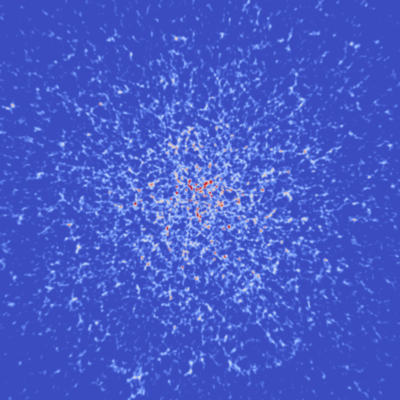
This figure shows the effect of global cosmological expansion on the observation of density field. The effect corresponds to a global radial geometrical distortion. The color palette goes from blue (lowest density) to white and red (highest density).